[ad_1]
August 24, 2023

At Spotify, we run a whole lot of A/B exams. Most of those exams comply with an ordinary design, the place we assign customers randomly to regulate and remedy teams, after which observe the distinction in outcomes between these two teams. Usually, the management group, often known as the “holdout” group, retains the present expertise, whereas the remedy group experiences a distinction: a brand new function, a change to an algorithm, or a redesigned person expertise.
Sometimes, nonetheless, there are considerations about working a “standard” A/B check. For occasion, we might wish to perceive the impression of a function that has already been rolled out to all the person base, or we might wish to run a advertising marketing campaign alongside a function launch. The advertising marketing campaign would then direct customers to the brand new function, however customers within the management group wouldn’t be capable of discover it, as they don’t have entry to the function. This makes for a nasty person expertise. Another concern is that the brand new function may need a sharing or messaging part the place customers can work together with one another. If customers can share a facet of the function with others, we ideally need all of those customers to have entry to the function, which makes it tough to have a management group. Lastly, we additionally launch experiences at Spotify that customers stay up for and count on, such because the annual Wrapped marketing campaign.
If we are able to’t embody a management group in these conditions, how can we measure the function impression? One doable reply is to run an encouragement design. The core concept of an encouragement design is to assign the remedy to all the inhabitants that we’re testing on, however randomize the encouragement to make use of the function. For occasion, if we wish to check a brand new function, we’ll simply allow this new function for all customers. However, we’re nonetheless including a component of randomization: for the remedy group, we’d place a banner to make use of the brand new function on the Home web page, whereas within the management group we don’t embody such an encouragement. This randomized encouragement can be utilized to compute a conditional common remedy impact utilizing an instrumental variables (IV) estimator.
Compared to different causal inference methods that depend on observational knowledge, an encouragement design has the benefit that it’s nonetheless primarily based on randomization. It does, nonetheless, estimate a special amount in comparison with an ordinary A/B check, and it requires just a few assumptions. I’ll focus on how the encouragement design compares to common A/B testing, what the pitfalls of interpretation are, and why the statistical properties of the IV estimator are vital when working an encouragement design.
Three forms of experiments
Encouragement designs share a whole lot of similarities with “standard” A/B exams. To make these connections clear, we’ll first check out A/B exams with full compliance adopted by A/B exams with one-sided noncompliance. A/B exams with full compliance are the gold commonplace and pose only a few problems with interpretation if appropriately carried out. In follow, lots of our A/B exams, nonetheless, have one-sided noncompliance, which complicates the scenario. An encouragement design is a generalization of those two sorts, the place we flip noncompliance right into a function of the experimental design.
Full compliance
In a perfect A/B check, we randomly assign every person to a remedy or a management group. All customers within the remedy group expertise the remedy, and all customers within the management group don’t expertise the remedy (see Figure 1).
| Random project (Z) | Treatment standing (D) |
| Treatment | Treated |
| Control | Untreated |
We cope with A/B exams with full compliance, for example, once we change the algorithm that powers Spotify’s Home web page or the search algorithm. Although not all customers use Home or Search, we are able to merely limit the inhabitants to teams which have used these options through the experiment.1
What makes these exams the gold commonplace is that we have now just one group of customers, which we name the “compliers.” Users within the remedy group adjust to their project and are handled, and customers within the management group additionally adjust to their project, and are untreated.
For the subsequent sections, it’s helpful to introduce some definitions:
- Z is an indicator (0/1) variable that signifies whether or not a person was assigned to the remedy or the management group.
- D is an indicator (0/1) variable that signifies whether or not a person was handled.
- Y is the end result we care about.
In an A/B check with full compliance, identifies the common remedy impact (ATE), that’s the causal impact of the function on the end result.
One-sided noncompliance
In follow, many A/B exams do not need good compliance, as a result of we frequently don’t drive customers to really take the remedy. This might be the case, for example, once we add a brand new function to the app. This signifies that we have now two forms of customers within the “Treatment” group — those who truly use the function (handled customers2) and those who don’t. Additionally, we additionally count on that customers that choose into the remedy usually are not randomly chosen — absolutely, for example, extra engaged customers usually tend to check out a brand new function. This setup is proven in Figure 2. Note that there isn’t any longer a 1:1 relationship between Z and D, as there are handled and untreated customers within the “Treatment” group.
| Random project (Z) | Treatment standing (D) |
| Treatment | Treated |
| Untreated | |
| Control | Untreated |
In this case, the amount not identifies the ATE, however the intent-to-treat impact (ITT). From a enterprise perspective, the ITT is vital as a result of it provides a sign of the causal impact of the whole product expertise — it consists of the mixed impact for customers and non-users of the function, in comparison with the management group. However, this often signifies that the ITT is far smaller than the causal impact of the function, as a result of the ATE is diluted by these customers that haven’t been complying with the project. For occasion, only a few customers might have truly used the function, however the function may match very effectively for these customers. Generally, subsequently, it will be helpful to know each the ITT and the causal impact of the function.
With compliance points, we are able to’t recuperate the ATE, the true causal impact of the function on the end result. However, underneath sure assumptions, we are able to recuperate the ATE for the compliers:
The components divides the ITT by the estimated proportion of compliers. For occasion, if the ITT is 1, and 50% of customers within the remedy cell had been truly handled, we’d estimate the causal impact for compliers to be 2. The logic right here is that the ITT is diluted by the noncompliers. Of course, this doesn’t work if there are not any compliers, as a result of then we’d divide by zero. The validity of this method hinges on just a few assumptions that shall be mentioned under.
The amount is often known as the native common remedy impact, LATE (native as a result of it applies solely to compliers) or the complier common causal impact (CACE). The estimator is named an instrumental variables estimator.
Encouragement design
In an encouragement design, we go one step additional and permit noncompliance in each the remedy and the management group. The random project is now not about function availability, however about an encouragement to make use of the function. This could possibly be, for example, a distinguished banner someplace within the app that’s accessible solely to the remedy group. In an encouragement design, we consider noncompliance not as a bug, however as a function. This setup is proven in Figure 3.
| Random project (Z) | Treatment standing (D) | Group composition |
| Treatment (inspired) |
Treated | Always-takers and compliers |
| Untreated | Never-takers and defiers | |
| Control (not inspired) |
Treated | Always-takers and defiers |
| Untreated | Never-takers and compliers |
Again, the ITT is . This is now measuring the impact of the encouragement on the end result, so it’s clearly not what we’re all for. The logic to calculate
is similar as above, however we’ll now present methods to derive the components. For this, it’s helpful to consider 4 distinct teams of customers:
- Always-takers: These are customers who use the function no matter whether or not they’re assigned to the remedy cell or the management cell.
- Compliers: These customers use the function if they’re assigned to the remedy cell, however don’t use the function if they’re assigned to the management cell.
- Never-takers: These are customers who by no means use the function no matter whether or not they’re assigned to the remedy cell or the management cell.
- Defiers: These are customers who at all times do the other of what’s supposed: When they’re inspired to make use of the function, they don’t use it, however after they aren’t inspired, they use the function.
In follow, we are able to by no means inform which group a person belongs to, as a result of we solely observe one state of the world. For occasion, customers that had been assigned to the remedy cell and had been truly handled could possibly be both always-takers or compliers.
Given that we have now 4 mutually unique teams of customers, we are able to rewrite the ITT as a weighted common of the ITT inside the 4 teams:
the place refers back to the proportion of group i.
Additionally, we now make three key assumptions:
- There are not any defiers (monotonicity), i.e.,
.
- The encouragement doesn’t have an effect on the outcomes for always-takers and never-takers (exclusion restriction), i.e.,
.3
- The encouragement works (relevance), i.e.,
.
With these assumptions, the components above might be rearranged, as many phrases drop out:
We have now derived the instrumental variables (IV) estimator.4 Again, shall be undefined if there are not any compliers, as a result of then we’d divide by zero. Another strategy to put that is that if
, then our encouragement doesn’t work, and we have now no compliers by definition. If the encouragement is designed effectively, this, hopefully, received’t occur!
It is vital to emphasise that is a native common remedy impact (LATE), and, subsequently, solely applies for this subpopulation. This signifies that if, for example, your IV experiment had solely 5% compliers, then the LATE can even solely apply to those 5%, and we don’t study something concerning the remedy impact for the remaining 95% of the inhabitants. This can also be the explanation why IV estimators usually have greater commonplace errors — our statistical energy solely comes from a subset of the inhabitants. It is vital to comprehend that there are compliers in each the remedy and the management teams. The compliers within the management teams are compliers within the sense that they might have taken the remedy if we had inspired them.
An further drawback of interpretation comes from the truth that the compliers usually are not a well-defined inhabitants. An particular person is likely to be a complier in a single experiment, however a never-taker in one other carefully associated experiment. Whether it’s helpful to make inferences about compliers is a degree that’s contested within the literature on instrumental variables. Making inferences a few inhabitants that’s not outlined beforehand however outlined by the instrument itself is a weak spot of the encouragement design. However, relying on the precise examine, the compliers may additionally be precisely the inhabitants that’s of curiosity — specifically these customers that we are able to encourage to take up a sure conduct. Either manner, this issue of interpretation is a part of the trade-off we make with encouragement designs in comparison with conventional A/B exams.
A more in-depth have a look at the assumptions of the IV estimator
The commonplace assumptions that must be happy in any IV examine are the secure unit remedy worth assumption (SUTVA) and the randomization of the remedy (right here, the instrument). These are the identical assumptions as in some other A/B check, so we won’t delve deeper into these.
The different assumptions might be encoded in a DAG, which is proven in Figure 4.
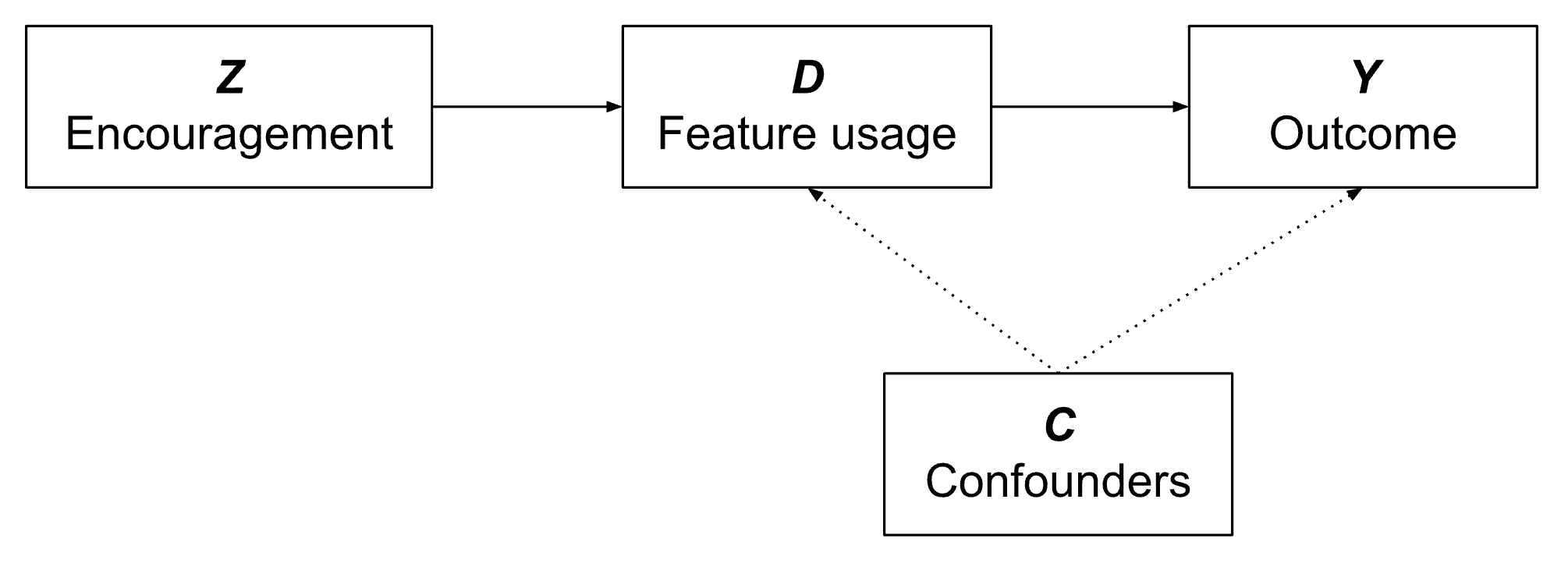
Note: Dashed strains point out probably unobserved relationships.
The identification drawback we’re coping with is represented by the confounders, C. Because these are usually unmeasured, we can not merely break up the pattern by function utilization and study concerning the causal impact of the function D on the end result Y. In an ordinary A/B check, we’d randomize D, which severs the trail from C to D, and identifies the causal impact. In the instrumental variable setting, nonetheless, we randomize Z.
Three assumptions round Z then must be happy:
1. Monotonicity: This signifies that the instrument at all times has to work in the identical path for all people. Another strategy to state that is that there are not any defiers. This assumption might be fairly believable in lots of settings, or at the least we are able to assume that the variety of defiers ought to be pretty low. However, it’s often not too exhausting to inform a narrative the place defiers are current.
2. Exclusion restriction: This assumption is visually depicted within the DAG within the sense that there isn’t any path between Z and Y besides by the function D. Another strategy to state that is that the encouragement itself mustn’t have an unbiased causal impact on the end result Y. A violation of the exclusion restriction is just not unlikely if the encouragement may be very intrusive, particularly for the never-takers who weren’t within the function within the first place. In follow, the exclusion restriction is usually the most important problem in defending the interpretability of an IV estimate.
3. Relevance of the instrument: This is depicted within the DAG as a direct arrow between Z and D. Another strategy to state that is that we would like function utilization to be greater within the inspired group in comparison with the non-encouraged group. Luckily, this assumption is definitely testable. In a broader sense, additionally it is vital that the impact of Z on D is numerically not too small, that’s, the encouragement ought to be substantively related as effectively. If this isn’t the case, you could run into the “weak instrument problem”, which may result in giant commonplace errors and, extra significantly, to a big bias within the IV estimator. If the instrument is weak, a bigger pattern dimension can typically make up for a few of the weak spot, nonetheless, which is nice information in settings the place the pattern dimension is much less of a difficulty. Some textbooks give the recommendation that the F statistic of the regression of D on Z ought to be at the least 10, however ideally it’s far bigger than this.
In encouragement designs, the second and third assumptions are considerably in opposition. On the one hand, we have to design an encouragement that’s extremely efficient (related) in producing an uplift for function utilization. On the opposite hand, a extra intrusive encouragement may additionally alter person conduct in surprising methods and thereby immediately affect the end result. These two necessities must be balanced when designing experiments with an encouragement design and, ideally, incorporate prior substantive data on person conduct and encouragement results.
If there’s a concern that the exclusion restriction is just not absolutely happy, it’s doable to do a sensitivity evaluation. For occasion, one can assume a small unfavourable impact for the never-takers (obtained, for example, from associated experiments) and check how this impact would affect the LATE.
Standard error of the IV estimator
The logic of the IV estimator is to make use of solely a part of the variance in D to estimate the remedy impact on the end result Y. The a part of the variance that we’re utilizing is that half that’s attributable to Z. However, utilizing solely a part of the variance of D additionally signifies that we’ll have greater commonplace errors (in comparison with an ordinary A/B check).
A full derivation of the usual error of the IV estimator is outdoors the scope of this weblog submit, however the last components remains to be helpful to construct instinct. To calculate the usual error, first outline a residual. This residual is much like the residual of a regression of Y on D, however removes solely the variation that’s attributable to the remedy impact of the compliers that runs by Z. For this, outline because the noticed worth of Y for particular person i, and
because the noticed worth of D. Then, let
characterize the residual for the ith particular person:
the place and
are pattern averages of
and
, respectively.
We can take into consideration ui as every part from Y that’s left over after we account for the causal impact of function utilization on our end result of curiosity. The variance of the IV estimator is then:
We need this amount to be low. There are 3 ways to attain this:
1. Increase the pattern dimension, n.
2. Reduce the numerator: This is tough, as a result of it is determined by the dimensions of , the causal impact we wish to estimate. Generally, we have now decrease variance when our causal impact is stronger. The greater the residual variance, the more durable it’s to measure the impact. This is similar drawback that we have now in any A/B check — we’d like extra knowledge once we wish to measure a small impact.
3. Increase the dimensions of the denominator: The denominator measures the energy of the instrument, and can develop because the distinction between and
grows. If the denominator is low, we might have a “weak instrument” drawback.
To make IV designs effectively powered, we require a big pattern dimension and an efficient instrument. Ideally, we have now excessive function uptake within the encouragement group, however low function uptake within the management group.
Conclusion
Encouragement designs and IV estimators might be helpful instruments in conditions the place an ordinary A/B check is just not doable or not fascinating. The upsides of an encouragement design (permitting all customers entry to a function and making advertising doable) must be balanced with the downsides (doable violations of the exclusion restriction, the restricted interpretability of the LATE, and the upper necessities to achieve statistical energy).
One large benefit of the encouragement design framework is that it sharpens the excellence between a function and its entry factors: the function in itself would possibly work very effectively, however provided that we get it in entrance of the proper subset of customers, specifically the compliers and always-takers. The complete rollout impression of a function can then be decomposed as a product of the LATE and the proportion of customers utilizing the function, and we are able to assume individually about optimizing every issue.
This overview of encouragement designs and IV estimation simply scratches the floor of an unlimited literature. For occasion, we assumed a binary instrument (inspired or not inspired) and a binary remedy (used the function or not), however each the instrument and the remedy will also be steady — we may take into consideration totally different strengths of encouragement, for example. A steady instrument permits a wider vary of statistical methods. Continuous devices, at the least in concept, additionally enable for the estimation of heterogeneous remedy results. Some extensions of the essential IV framework offered listed here are mentioned within the assets given within the “Further reading” part under.
This submit mentioned IV estimation largely within the context of encouragement designs, however their applicability extends past this context. For occasion, IV estimation can be utilized to right for noncompliance if there have been technical issues with establishing an experiment (e.g., sample-ratio mismatch). IV estimation will also be used to estimate the causal impact of one thing that’s tough to control immediately. For occasion, at Spotify we are sometimes within the results of upper consumption on totally different outcomes, however we are able to’t A/B check on consumption immediately. However, if we discover a legitimate instrument for consumption (e.g., an encouragement in order that customers devour extra) that’s not immediately associated to the end result in query, then we are able to recuperate the causal impact of consumption on an end result.
Further studying
For an approachable introduction to IV, see Chapters 21.1 and 21.2 in Andrew Gelman, Jennifer Hill, and Aki Vehtari (2020): Regression and Other Stories (PDF accessible on-line).
For a extra in-depth remedy, see superior textbooks similar to Stephen L. Morgan and Christopher Winship (2014): Counterfactuals and Causal Inference (extremely really helpful!) or Miguel A. Hernán and James M. Robins (2020): Causal Inference: What If (PDF accessible on-line).
For a remedy that features code examples in Python and R, see Scott Cunningham (2021): Causal Inference: The Mixtape (on-line model).
Some on-line assets:
Notes
- Another strategy to say that is that we are able to filter out the noncompliers of each the remedy and the management teams, which isn’t doable within the different two forms of A/B exams. Of course, if we wish to calculate the rollout impression from such an experiment, we’d nonetheless have to keep in mind the proportion of customers that use Home or Search.
- We outline “treated users” as customers which have used the function. However, “untreated” customers would possibly nonetheless be handled within the sense that they’ve seen the entry factors for a function, which could additionally alter their conduct. The assumption that these customers are unaffected by the entry factors is named the exclusion restriction.
- Saying that the ITT is zero for always-takers and never-takers doesn’t imply that these customers can’t have a remedy impact when it comes to D — it simply signifies that the encouragement doesn’t have something to do with altering their end result. However, it’s unimaginable in our design to say something concerning the remedy impact when it comes to D for these teams as all always-takers have taken the remedy and all never-takers haven’t taken the remedy.
- If you’re questioning concerning the denominator within the final expression, right here’s the derivation: due to random project, we can have the identical proportion of always-takers, never-takers, and compliers in each the “Treatment” and “Control” cells. Hence, the proportion of always-takers in our inhabitants might be estimated by E[D | Z = 0] (proportion handled within the “Control” group). Similarly, the proportion of never-takers might be estimated by 1 – E[D | Z = 1] (proportion untreated within the “Treatment” group). The proportion of compliers have to be what’s left over after subtracting these two teams, which is precisely what we have now within the denominator.
Tags: experimentation
[ad_2]